Welcome!

This blog accompanies A Student’s Guide to Python for Physical Modeling by Jesse M. Kinder and Philip Nelson.  The book is now in its second edition!

A Student’s Guide provides an introduction to the Python computer language and a few libraries (NumPy, SciPy, and PyPlot) that will enable students to get started in physical modeling. Some of the topics covered include the following:

  • basic Python programming
  • importing and exporting data
  • numerical arrays
  • 2D and 3D plotting
  • Monte Carlo simulations
  • numerical integration
  • solving ordinary differential equations
  • symbolic mathematics
  • animation
  • image processing
  • Python classes
  • version control with Git

You can have a look at the Table of Contents.

On this Web site, you will find data sets, code samples, errata, additional resources, and extended discussions of the topics introduced in the book.

Enjoy!
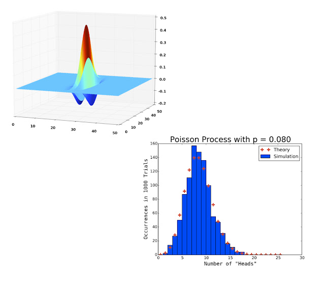
Plots created with NumPy and PyPlot.

Comments

Popular posts from this blog

Paths in Python

How do you get your Python interpreter to find modules that are not located in your current working directory? The answer is … you tell it where to look. When you type something like from my_module import my_function Python searches a collection of directories (i.e., folders) on your computer. If the directory containing <my_module.py> is not in this collection, you will receive an ImportError . This can be frustrating if you know the file exists, and even more so if you know where it exists. In this post, we will take a brief look at how to add paths to the collection of directories searched by Python. Paths A path is essentially a set of directions to a file: /Users/username/modules/my_module.py [Mac OS X, Linux] C:\modules\my_module.py [Windows] It tells your operating system how to navigate from a fixed starting point — the “root directory” / in Unix-based systems, or C:\ in Windows — through a collection of folders to the de

Raising a Figure Window to the Foreground

This post describes a utility function that will raise a plot window to the foreground of your screen. The function will only work with the Qt graphics backend, so I will start with a brief overview of graphics backends. If you just want to use the function as a black box, you can do the following: Set the Graphics Backend to “Qt” in the Spyder preferences menu. Copy this function into your working directory. Graphics Backends You may have have written a script to produce precisely the data you need, but a lot of processing is required to transform these numbers into a figure. You need to create a plot window, draw a figure inside of it, and manage all of the attributes that control a figure’s appearance: title, axis labels, line widths, colors, tick marks, etc. All of this happens in the background when you type a command like plt.plot(x,y) . A graphics backend is the software that Python uses to physically draw a figure on your computer screen. If you have already import

Illuminating Surface Plots

Matplotlib provides functions for visualizing three-dimensional data sets. One useful tool is a surface plot. A surface plot is a two-dimensional projection of a three-dimensional object. Much like a sketch artist, Python uses techniques like perspective and shading to give the illusion of a three-dimensional object in space. In this post, I describe how you can control the lighting of a surface plot. Surface Plots First, let’s look at some of the options available with the default three-dimensional plotting tools. This script will create a surface plot of a Bessel function. Its ripples will emphasize the effects of lighting later. import numpy as np import matplotlib.pyplot as plt from mpl_toolkits.mplot3d import Axes3D # Import 3D plotting tools. from scipy.special import jn # Import Bessel function. # Define grid of points. points = np.linspace(-10, 10, 51) X, Y = np.meshgrid(points, points) R = np.sqrt(X**2 + Y**2) Z = jn(0,R) # Create 3D surface plo